The issue of sampling was briefly mentioned in the context of the number of detector pixels in the seeing disc of a star when using a focal reducer. In this section we shall look at why sampling is an essential consideration when designing astronomical instruments, including both imagers and spectrographs.

Sampling is the process of converting a continuous signal, in this context an image or spectrum in the focal plane of an astronomical instrument, into a discrete signal, by selecting values at evenly-spaced points in the focal plane. This latter function is performed by the pixels in a detector. The question is, how finely spaced (i.e. how big) do the detector pixels have to be in order to faithfully recover the input signal? The solution is given by the Nyquist sampling theorem, which states that:

The sampling frequency should be greater than twice the highest frequency contained in the signal.

In other words, if the smallest feature in an image or spectrum has a dimension of x μm (i.e. the highest spatial frequency is 1/x cycles [or "features"] per μm), then the pixel size must be no larger than x/2 μm (i.e. the sampling frequency must be greater than 2/x cycles per μm) in order to detect all of the information in the image or spectrum.

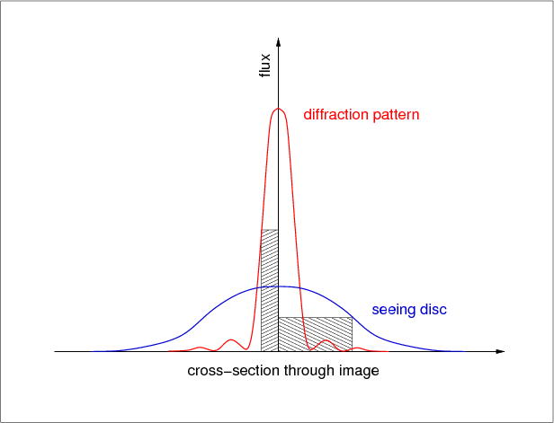
The smallest real features present in an image will be those at the resolution limit, which is normally given by the seeing. If the seeing is 1", the Nyquist sampling theorem tells us that we would require 2 pixels across the seeing disc in order to sample the image optimally, i.e. the plate scale should be 0.5 "/pixel. This situation is shown schematically in figure 74. If we have more than 2 pixels across the seeing disc, the image is said to be oversampled, whereas if we have less than 2 pixels across the seeing disc, the image would be undersampled. A degree of oversampling is normally acceptable (for example to cope with the fact that the size of a pixel across the diagonal is greater than across a side), but too much oversampling results in a needlessly reduced field of view. Undersampling, however, is rarely desirable, as it means that the image recorded by the detector is of a lower spatial resolution than the image delivered by the telescope, and undersampling can also cause problems during data reduction. The only occasions when undersampling might be desirable is if increasing the field of view or decreasing the contribution of detector (readout) noise is of paramount importance.

figure 74:

Nyquist sampling of stellar profiles. Two profiles are shown - one at the theoretical diffraction limit of the telescope and another smeared into a seeing disc. The narrow hatched box, which is equal to half the FWHM of the Airy disc in the diffraction-limited profile, indicates the pixel size required to sample the profile at the Nyquist frequency. The wider hatched box, equal to half the FWHM of the seeing-limited profile, shows the pixel size required to sample the seeing disc at the Nyquist frequency.

 

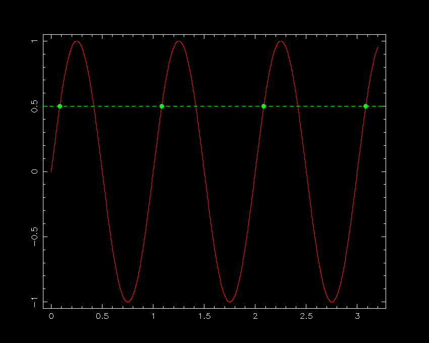
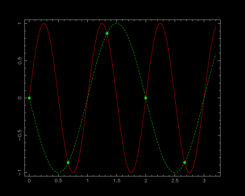
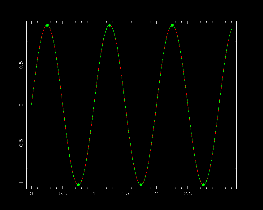
To understand why there is a critical sampling frequency that determines whether or not an image or spectrum is optimally sampled, it is easiest to consider the case of a signal consisting of a sine curve, as shown in figure 75. Sampling the continuous sine curve only once per cycle would not reveal any variation at all (left-hand panel of figure 75). Sampling at 2/3 times the period of the sine curve (central panel of figure 75) would begin to reveal variation, but one would be fooled about its period. (This effect is known as aliasing and is most commonly seen in movies of the spokes in a rotating wheel, where an alias of the true period of the wheel is produced by the frame rate of the camera being below the Nyquist frequency). Sampling the sine curve twice per cycle (right-hand panel of figure 75), as suggested by the Nyquist sampling theorem, is the minimum required to detect all of the peaks and troughs in the signal. Note, however, that one could be unlucky and still hit upon only the points at which the sine curve crosses the x axis - this is why the Nyquist sampling theorem states that the sampling frequency should be greater than twice the highest frequency contained in the signal, and why, strictly speaking, the theorem only applies to an infinitely long signal.

figure 75:

A signal consisting of a continuous sine curve with unit period is shown in red. Left: Sampling only once per cycle (green dots) results in the signal being wongly interpreted as a constant (green dashed line). Centre: Sampling every 2/3 of a cycle results in the signal being interpreted as a sine curve, but of an incorrect period. This is aliaising. Right: Sampling twice per cycle, as suggested by the Nyquist theorem, allows the original signal to be recovered.

   

An example of how consideration of the Nyquist sampling theorem is important for the design of an imager is given in the example problems.