Determining the uncalibrated signal from a source in an image is usually a three-step process. The first step is to measure the centre of the source, which for the rest of this discussion we shall assume is a star. The second step is to estimate the sky background at the position of the star. The third step is to calculate the total amount of light received from the star.

centroiding

The first step - accurately determining the centre of the star in the image (or centroiding) - is usually achieved by adding up the light from the star along the rows and then the columns of the CCD, giving a one-dimensional stellar profile in the x direction and another in the y direction. The resulting profiles, which are known as Point Spread Functions or PSFs are then fit with a one-dimensional Gaussian (or similar) function, akin to those shown in figure 80. The position of the centre of the Gaussian fit is then used as an estimate of the centre of the star, which can change as a function of time due to guiding and seeing variations. This technique can fail in crowded fields, or if the stellar PSF is very faint or highly non-Gaussian; a number of more complex centroiding techniques exist for such cases.

sky background

Every pixel containing light from the star also contains light from the night sky. The great advantage of imaging photometry is that the level of this sky background can be estimated simultaneously with, and at almost the same position on the sky as, the star. To determine the sky background, the usual procedure is to measure the signal in an annulus centred on the star, as shown in figure 81. Such a measurement ensures that, to first order, any gradient present in the sky background is cancelled out. Clearly, the inner radius of the annulus must be large enough to avoid contamination with light from the star at the centre, and the outer radius must be large enough to ensure that the annulus contains sufficient pixels for a robust estimate of the sky signal.

Unfortunately, the annulus is unlikely to contain signal from the sky alone. There will also be contributions from cosmic rays, hot pixels, faint stars, and the wings of the PSF of the central star. All of these will add a positive skew to the histogram of pixel values in the annulus. The mean of these pixel values will then not be an accurate representation of the sky background. Instead, the sky level is usually determined using a more robust estimator, such as the median (i.e. the central value) or a clipped mean, as shown in figure 79.

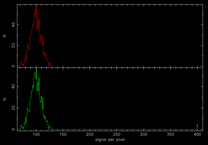
figure 79:

The top histogram shows the distribution of the signal in a sky annulus containing 1000 pixels. The mean and median of this distribution have the same value, 99.5, which represents the background sky level. The bottom histogram shows the distribution of the signal in the same sky annulus, but with the addition of 7 cosmic rays, each with a signal of 400, resulting in the small peak at the right-hand side. This skews the mean of the distribution to a value of 101.8, but the median effectively rejects these outliers and remains at the true sky level of 99.5. Therefore, adopting the mean rather than the median would result in a 2% error in the sky signal.

extraction

There are two ways in which the total signal from a star can be extracted from an image. The first is profile fitting, where the star is fitted with a function that closely matches its shape (e.g. a Gaussian, modified Lorentzian, or Moffat profile), as shown in figure 80, and the function is then integrated to calculate the area underneath it. It is also possible to use the bright stars in an image to define an empirical profile, which is then fitted to the star of interest. Profile-fitting techniques are mainly used for faint stars and/or crowded fields, and they often assume that all the stars in an image have the same PSF. The latter assumption can be erroneous in the presence of off-axis aberrations or seeing-induced spatial variations in the PSF.

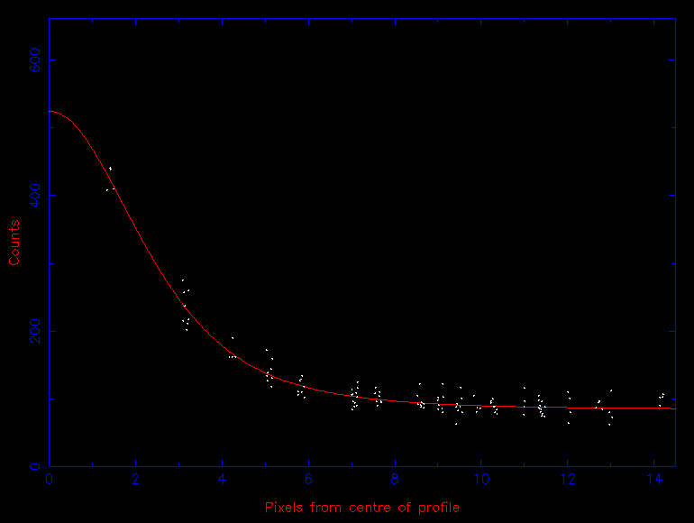
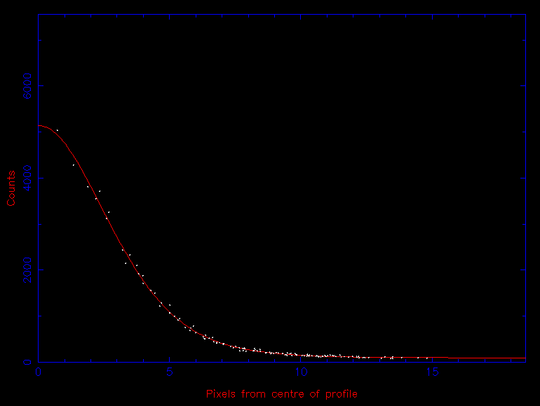
figure 80:

Left: Moffat fit to the faint star (aperture 1) in figure 81. Right: Moffat fit to the bright star (aperture 2) in figure 81. Note how their FWHM are almost identical, even though the bright star appears to cover more pixels than the faint star in figure 81. The background sky level is given by the vertical offset of the fit from the x axis.

 

The second, more commonly-used approach to extracting photometric data is known as aperture photometry. In this case, a software aperture, usually a circle or ellipse, is centred on the star, as shown in figure 81. The total signal from the star can then be calculated by summing the signal from each pixel that falls inside the aperture, and then subtracting the previously-determined sky background from each pixel.

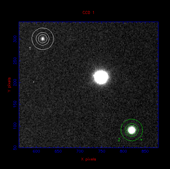
figure 81:

Aperture photometry from a CCD image. The target, an eclipsing cataclysmic variable star, is labelled as aperture 1. The non-variable comparison star is labelled as aperture 2 (in green). The unmarked bright star is saturated and hence unusable. The inner circle defines the total signal from the target. The annulus defined by the two outer circles is used to calculate the signal from the sky.

The optimum aperture size to use depends on the brightness of the star. As the aperture size is increased, an increasing fraction of the star light will obviously be included in the sum. However, the increasing aperture size also allows in extra light from the sky, as well as extra detector noise, both of which will degrade the signal-to-noise ratio. Hence, as the aperture size is increased, a point will come when the combination of the extra sky and detector noise will dominate over the extra light included from the star. If one is interested in the total signal from the star, a common procedure then is to plot a curve of growth, which is a plot of the signal from the star as a function of aperture radius. This will asymptotically reach a maximum value that can be estimated from the graph.

If, instead, one is interested in the relative signal from the star, e.g. when studying variability, then measuring the total signal is not important. In this case, the signal from the variable star (aperture number 1 in figure 81) is divided by the signal from a nearby, non-variable comparison star on the same CCD image (aperture number 2 in figure 81). (Equivalently, from m₁-m₂ = -2.5 log₁₀(F₁/F₂), the magnitude of the comparison star is subtracted from the magnitude of the variable star.) This technique is known as differential photometry and is used to correct for transparency and seeing variations, which might otherwise mimic the intrinsic variations of the variable star. The resulting plot of the relative signal from the variable star versus time is known as a light curve, an example of which is shown in figure 82. The optimum-sized aperture to use in this case is one which minimises the scatter in the light curve, which can be deduced by trial and error by changing the aperture size so as to minimise the standard deviation in a flat portion of the light curve. It is important to note here that the same sized aperture must be used for both the variable star and the comparison star, as the fraction of the total signal in an aperture of a given size is the same regardless of the brightness of a star (as demonstrated in figure 80). Hence, if the seeing increases, the fraction of light lost from the apertures of both stars is the same and dividing one by the other will then correct for the resulting signal variation.

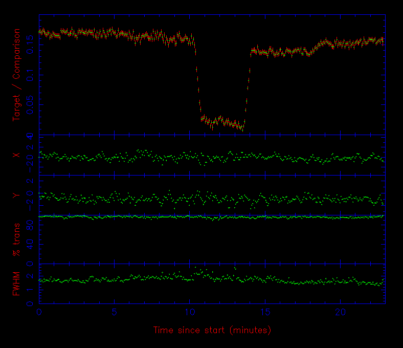
figure 82:

Differential photometry obtained with ULTRACAM. The top panel shows the light curve of an eclipsing cataclysmic variable: the signal from aperture 1 (the variable) in figure 81 is divided by the signal from aperture 2 (the comparison star) and plotted as a function of time. The two panels below this show the centroid of aperture 2 in both the x and y directions. The units are pixels, where 1 pixel = 0.3" and zero corresponds to the position of the star in the first CCD image. The variability in the centroid is due to the autoguider correcting the telescope tracking errors. The panel below this shows the sky transparency, as determined from the signal of the comparison star, where 100% represents the maximum signal observed. The bottom panel shows the seeing (i.e. the FWHM of the PSF) in arcseconds, as measured from aperture 2.