| photon statistics |
|
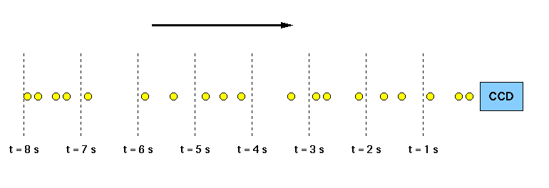
The vast majority of astronomical sources produce photons via random processes distributed over vast scales. Therefore, when these photons arrive at the Earth, they are randomly spaced, as illustrated in figure 115. The number of photons counted in a short time interval will vary, even if the long-term mean number of photons is constant. This variation is known as shot noise. It represents the irreducible minimum level of noise present in an astronomical observation.
| figure 115: |
Photons from a faint, non-variable astronomical source incident on a
CCD detector. Because the signal is low in this example, it is easy
to see that there is a substantial variation in the number of photons
detected in each 1 s time interval.
|
If one plots a histogram of the number of photons arriving in each time interval, the resulting distribution is known as a Poisson distribution, as shown in figure 116. Poisson statistics are applicable when counting independent, random events which occur, when measured over a long period of time, at a constant rate. The Poisson distribution is therefore applicable to the counting of photons from astronomical sources, the counting of photons from the sky, or the production of thermally-generated electrons in a semi-conductor (i.e. dark current).
| figure 116: |
Poisson distributions for mean values of μ = 1, 4 and 10.
Pr is the probability of observing r events.
For each value of μ, the mean of the distribution is at μ
and the standard deviation is μ0.5. As μ increases,
the Poisson distribution approaches the Normal distribution. |
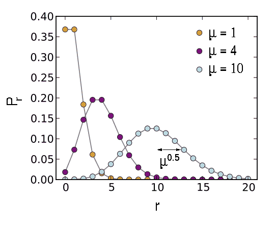
An important property of the Poisson distribution is that the standard deviation is equal to the square root of the mean, as indicated in figure 116. Hence if the mean is μ then the error on the mean is μ0.5. For example, if μ = 10, then the fractional error is μ0.5/μ = 31.6%. If μ = 100, then the fractional error is μ0.5/μ = 10%. This shows that as more photons are counted, the noise becomes a smaller fraction of the signal, i.e. the signal-to-noise ratio improves. For more examples, see the example problems.
removed from course: proof that the variance of the Poisson distribution is equal to the mean.