Active optics only counteracts the effect of gravity and other deformations on the telescope mirrors, and operates on timescales of tens of seconds. Correction for the effects of the Earth's atmosphere, on the other hand, is the realm of adaptive optics, which operates on timescales of hundredths of a second. Before we describe the basic principles of adaptive optics, it is necessary to define three important terms that characterize the effects of turbulence in the Earth's atmosphere on a wavefront propagating through it: the Fried (pronounced free-d) parameter, the coherence time and the isoplanatic angle.

fried parameter

r₀ ^6/5

figure 62:

Schematic showing how the Fried parameter, r0, coherence time, t0 = t2 - t1, and isoplanatic angle, 0, are defined.

We have already seen that the size of a diffraction-limited image is proportional to /D. We have also seen that large telescopes (defined here as those with D >> r₀) are not limited by diffraction, but by the seeing. In fact, the size of a seeing-limited image is proportional to /r₀. Hence the seeing in a large-aperture telescope is proportional to ^-1/5. So, for example, if the seeing when observing at 500 nm is 1", it would be ~0.7" when observing in the near-infrared at 2.5 m.

coherence time

The turbulent cells responsible for distorting the plane wavefronts from a star generally evolve on longer timescales than the time it takes the wind to move a cell by its own size. Hence it is the wind velocity, v, at the altitude of the turbulence that determines the temporal variation of the wavefronts entering the telescope, as shown in figure 62. A turbulent cell would move its own size in a time t₀ = t₂ - t₁, given by

t₀ = r₀ / v.

At a good observing site on a typical night, v = 10 m/s and r₀ = 10 cm at ₀ = 500 nm. Hence t₀ = 10 ms. Detailed arguments lead to a more accurate version of this equation: t₀ ~ 0.314 r₀ / v. t₀ is known as the coherence time and indicates the timescale on which the wavefront sensor and deformable mirror of an adaptive optics system must operate. The dependence of t₀ on r₀ implies that adaptive optics correction in the infrared can be much slower (and hence is easier) than in the optical.

isoplanatic angle

Another parameter of importance in adaptive optics is the isoplanatic angle, ₀. Suppose that there are two stars close together on the sky. What angle would these two stars have to be separated by in order for them to pass through approximately the same turbulent region of the atmosphere? Figure 62 shows that this can be estimated from the angle over which the turbulence pattern is shifted by a distance of only r₀, in which case the beams from the two stars would share a substantial fraction of the turbulent region (shaded in yellow). Assuming that the turbulent layer is at an altitude h above the telescope, the isoplanatic angle is hence given by

₀ = r₀ / h.

At a good observing site on a typical night, h = 10 km and r₀ = 10 cm at ₀ = 500 nm. Hence ₀ = 10^-5 radians, which is ~2". Detailed arguments lead to a more accurate version of this equation: ₀ ~ 0.314 r₀ / h. The isoplanatic angle determines the area on the sky over which adaptive optics correction is effective. The dependence of ₀ on r₀ implies that much wider fields (and hence more extended objects) can be corrected with adaptive optics in the infrared than in the optical, making the technique much more attractive in the infrared. The increased isoplanatic angle in the infrared also means that many more natural guide stars are available, as discussed below.

basic principles of adaptive optics

The principles of adaptive optics correction are shown in figure 63. A plane wavefront from a star is corrugated by turbulence in the Earth's atmosphere. The diverging beam beyond the focal plane of the telescope is then made parallel using a collimator, and the collimated beam reflects off a deformable mirror, which is adjusted in shape to match that of the wavefront. As a result, the reflected wavefront becomes planar again, and the corrected beam is then focused and detected by a science camera. The shape of the deformable mirror is adjusted hundreds of times a second, using information provided by a wavefront sensor, which picks off the (unwanted) blue light in the beam using a dichroic beamsplitter. Note that the shape of the wavefront is independent of wavelength, which is why it is then possible to sense and correct at different wavelengths; you can think of an infrared wavefront as being a squashed (in phase) version of an optical wavefront.

figure 63:

Left: Schematic showing the principal components of an adaptive optics system. Right: Photograph showing the main components of the adaptive optics system on the 3m Shane Telescope at Lick Observatory, California: the deformable mirror (DM), the science camera (IRCAL) and the wavefront sensor.

wavefront sensors and deformable mirrors

The two most critical elements of an adaptive optics system are the deformable mirror and the wavefront sensor. There are many different types of each, so we shall concentrate here on the conceptually simplest: the Shack-Hartmann wavefront sensor and the segmented deformable mirror - see figure 64.

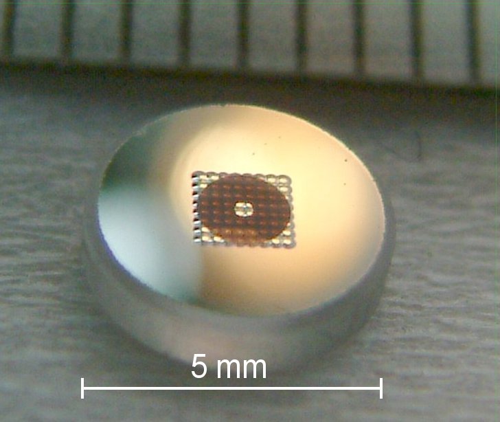
figure 64:

Photograph of a typical lenslet array for use in a Shack-Hartmann wavefront sensor. Photograph of a 76-element segmented deformable mirror, used in the NAOMI adaptive optics system on the 4.2m William Herschel Telescope (WHT) on La Palma.

The Shack-Hartmann wavefront sensor consists of a lenslet array which the corrugated wavefront is incident upon. A plane wavefront incident on the lenslet array would produce a regular series of spots on a high-speed detector in the focal plane. A corrugated wavefront, on the other hand, would produce irregularly spaced spots, where the tilt of each section of the wavefront can be determined by measuring the displacement of the spot from the fiducial position (defined by illuminating the lenslet array with a plane wavefront). This is shown in the left-hand and central panels of figure 65, together with a movie of data from a real Shack-Hartmann wavefront sensor.

figure 65:

Left: Schematic showing the principle of Shack-Hartmann wavefront sensing. Right: Movie of images obtained by the JOSE Shack-Hartmann wavefront sensor on the WHT when illuminated by a bright star (reload this page to restart the animation). The blank region at the centre is the shadow of the secondary mirror.

The tilt of the wavefront at each lenslet is then used to set the tilt of each corresponding element in the segmented deformable mirror (to a value equal to half of the tilt of the wavefront), so that the reflected wavefront becomes planar, as shown in the right-hand panel of figure 65. For accurate correction, it is essential that the delay between sensing the wavefront and adjusting the shape of the deformable mirror is no greater than the coherence time of the atmosphere, which is typically a few milliseconds in the optical part of the spectrum at a good astronomical site. Hence high-speed computer processors to measure the wavefront and move the mirror in a real-time correction loop are also an essential component of any adaptive optics system, as indicated in figure 63. It is also vital that the sizes of the lenslets, and hence the mirror segments, are well matched to the typical values of the Fried parameter at the observing site and wavelength of interest.

laser guide stars

In order for a Shack-Hartmann wavefront sensor to measure the tilts of a wavefront accurately, it is necessary to observe a bright point source to provide a sufficient signal-to-noise ratio in the short exposure times. It is possible that the science target itself can be used to sense the wavefront, e.g. if it has a bright, point-like central structure, such as an active galactic nucleus or young stellar object. Unfortunately, many astronomical targets are either faint, extended, or both. One way round this is to observe a bright star close to the target, but such a natural guide star would have to be within the isoplanatic angle of the target, otherwise the target and guide stars would be sampling different turbulence in the atmosphere (as shown in figure 62).

As calculated above, the isoplanatic angle in the optical part of the spectrum is only a few arcseconds, and this only increases to a few tens of arcseconds in the infrared. Hence only a very small fraction (or order 1-10 per cent) of the sky is actually correctable using adaptive optics with natural guide stars. The only way of significantly increasing the sky coverage is to generate an artificial guide star close to the target using a laser: a so-called laser guide star (figure 64).

figure 66:

Top left: Photograph of a laser beam emanating from the 8.2 m Very Large Telescope in Chile. Top right: Photograph of the laser guide star produced by the ALFA adaptive optics system on the Calar Alto 3.5 m telescope in Spain. The sodium beacon is the point-like image at the centre; the plume to the right is the Rayleigh back-scattered light. Bottom: A schematic illustrating the cone effect.

There are two types of laser guide star. The first, known as a Rayleigh beacon, uses the Rayleigh back-scattering of light from molecules in the lower atmosphere to produce an artificial star at altitudes of approximately 20 km. The second type is the sodium beacon, which uses a laser tuned to the yellow sodium D lines around 589 nm. This excites sodium atoms (deposited by micrometeorites) in the mesosphere at an altitude of approximately 90 km, which subsequently re-emit the light, producing an artificial star, as shown in figure 66.

Although much more more costly and complex than Rayleigh beacons, sodium beacons have one major advantage: they do not suffer as badly from the cone effect, resulting in superior adaptive optics correction. This is shown schematically in the bottom panel of figure 66, where it can be seen that the higher altitude of the sodium beacon means that it shares much more of the turbulence experienced by light from the star than the lower-altitude Rayleigh beacon. It is important to note, however, that a sodium laser focused to around 90 km altitude also produces an out-of-focus halo of light from Rayleigh back-scattering at lower altitudes. Fortunately, this halo can be ignored by using a pulsed laser and sensing the wavefront a few microseconds after the pulse has been launched; in this way, the scattered light from lower down in the atmosphere is rejected and only light which has travelled for several microseconds up to the sodium layer and back again is detected.

Since the laser passes twice through the turbulence, once on the way up and once on the way down, any overall tip and tilt of the wavefront, which manifests itself as overall image motion in the focal plane, is cancelled out. (The higher-order corrugations are not cancelled out as the laser is focused to a spot above the turbulent layer.) The stellar image, however, only passes once through the turbulence and hence will display this image motion which, if not corrected, will smear the image and thereby degrade the spatial resolution. Therefore, a natural guide star is still required for correction of this tip and tilt, but since only the image centroid needs to be measured, the guide star does not need to be anywhere near as bright, or lie as close to the target, as a natural guide star that is being used for higher-order corrections.

No matter which type of laser beacon is used, an artificial star is created that is (usually) above the typical altitudes at which turbulence occurs. The artificial star can be placed within the isoplanatic angle of the science target, resulting in sky coverage approaching 100% for adaptive optics (assuming a natural guide star is also available for the tip-tilt correction). Since the laser light is monochromatic, a simple notch filter can be used to direct all of the laser light to the wavefront sensor, leaving the rest of the light to be directed to the science detector.

adaptive optics in practice

We have already seen that the spatial resolution of a seeing-limited image is usually characterised by the full-width at half-maximum (FWHM) of a stellar profile, measured in arcseconds. This method becomes unreliable, however, as the spatial resolution approaches the diffraction limit, as measurement of the FWHM becomes complicated by the presence of diffraction rings. A more useful measure in this case is the Strehl ratio, which is the ratio of the intensity at the peak of the observed seeing disc divided by the intensity at the peak of the theoretical Airy disc, as shown in figure 67.

figure 67:

The seeing disc of a star superposed on the theoretical diffraction pattern. The Strehl ratio is the ratio of the peak intensities of the two profiles.

The Strehl ratio is the most commonly-used parameter to characterise the performance of an adaptive optics system. The Strehl ratio recorded by a telescope without adaptive optics is typically only a few per cent, but this can rise to over 50% if adaptive optics is used. The higher the Strehl ratio, the more the image is concentrated and hence the higher the spatial resolution. A higher Strehl ratio also means the image of a star is concentrated onto fewer detector pixels, minimizing the noise due to the sky background and the detector. In spectroscopy, a higher Strehl ratio implies that narrower slits can be used, which in turn means that the whole spectrograph can be made more compact.

Most large telescopes in the world are now equipped with adaptive optics systems. The most advanced such systems incorporate laser beacons and wavefront sensors/deformable mirrors with 1000+ elements, delivering diffraction-limited imaging in the infrared across most of the sky (see figure 68). However, diffraction-limited imaging on large-aperture telescopes is still not achievable in the optical. As discussed above, this is due to the lower values of the Fried parameter and coherence time, implying that an unfeasibly large number of adaptive elements and corrections per second would be required.

figure 68:

Adaptive optics in action: Top: Images of the binary star IW Tau without (left) and with (right) adaptive optics on the 5.1 m Hale Telescope in California. The separation of the two stars is 0.3". Bottom left: A movie showing images of a star taken with AO correction turned off and then on. Bottom right: Arguably the most famous AO result to date - a movie of the orbits of stars around the Galactic centre, taken using the 8.2 m Very Large Telescope in Chile, which was used to infer the presence of a supermassive black hole. The image is only 3 arcseconds across.